DATA Manipulation with R
Download data from Generalitat server and read the corresponding csv
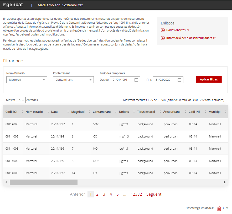
You have available the R code at my GitHub and you can edit in Visual Code Studio and to execute it using source instruction in RStudio.
# First you need to install some libraries to manipulate and analyse data
install.packages(c("openair","tidyverse", "lares"))
# Remember to edit the next line in order to use your city data
# Do not use my hourly data from Martorell
city<-read.csv('https://raw.githubusercontent.com/drfperez/openair/main/city.csv')
# You need to call tidyverse library in order to use pivot_longer
library (tidyverse)
# pivot_longer allows you to convert hour columns to hour rows
city1<-pivot_longer(city,cols=c(h01,h02,h03,h04,h05,h06,h07,h08,h09,h10,h11,h12,h13,h14, h15,h16,h17,h18,h19,h20,h21,h22,h23,h24), names_to="hour", values_to = "value")
# Delete unnecessary columns
city2<-city1[-c(1,2,4,6:16)]
# You need dplyr library from tidyverse to use pipe symbol %>% and combine two columns in one
library(dplyr)
city2 <- city2 %>% mutate(date=paste0(data, " ", hour))
# check the names of your columns
colnames (city2)
# delete some unnecessary columns
city2<-city2[-c(1,3)]
# reorder the columns
city2<-city2[,c(3,1,2)]
# rename the columns names
colnames (city2)<-c("date","pollutant","value")
# check changes of column names are correct
colnames(city2)
# check the class of city2
class (city2)
# convert city2 to a dataframe
city2 <- as_data_frame(city2)
# call lares library to find and replace some values including NA
library (lares)
city2<-replaceall(city2, c("T00:00:00.000 h01", "T00:00:00.000 h02","T00:00:00.000 h03","T00:00:00.000 h04","T00:00:00.000 h05","T00:00:00.000 h06","T00:00:00.000 h07","T00:00:00.000 h08","T00:00:00.000 h09","T00:00:00.000 h10","T00:00:00.000 h11","T00:00:00.000 h12","T00:00:00.000 h13","T00:00:00.000 h14","T00:00:00.000 h15","T00:00:00.000 h16","T00:00:00.000 h17","T00:00:00.000 h18","T00:00:00.000 h19","T00:00:00.000 h20","T00:00:00.000 h21","T00:00:00.000 h22","T00:00:00.000 h23","T00:00:00.000 h24"), c(" 01:00:00", " 02:00:00", " 03:00:00", " 04:00:00"," 05:00:00", " 06:00:00"," 07:00:00", " 08:00:00"," 09:00:00", " 10:00:00"," 11:00:00", " 12:00:00"," 13:00:00", " 14:00:00"," 15:00:00", " 16:00:00"," 17:00:00", " 18:00:00"," 19:00:00", " 20:00:00"," 21:00:00", " 22:00:00"," 23:00:00", " 00:00:00"))
# Call openair library to use built-in functions
library(openair)
# Convert date column from characters to dates
city2$date<-as.POSIXct(city2$date,"%Y-%m-%d %H:%M:%S", tz="Europe/Madrid")
# Check date column now is a date or POSIXct
class(city2$date)
# Convert pollutant column from numeric to factor
city2$pollutant<-as.factor(city2$pollutant)
# Check previous conversion is ok
class(city2$pollutant)
# To know the different levels of the factor pollutant in order to draw figures
levels(city2$pollutant)
# Create a figure with hour, day, week, month variations of pollutants
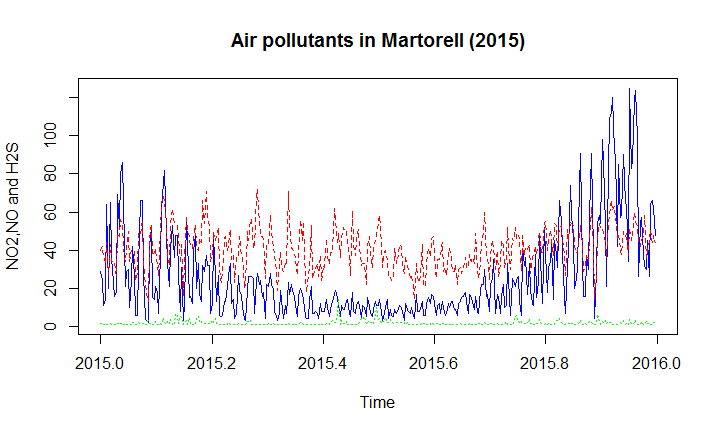
timeVariation(city2, pollutant=c("O3","NO2","H2S","NO","HCNM","CO","SO2","HCT", "NOX","PM10"), main="Air pollution in Martorell (1991-2022)")
# Create another view of the previous data centered in one pollutant
trendLevel(city2, pollutant = "H2S", main="Hydrogen sulfide evolution in Martorell")
# Calculate daily means from hourly data of poly
daily<-timeAverage(city2NO2,avg.time = "day")
View(daily)
# Create a calendar plot showing values of pollutants with colours
calendarPlot(daily, pollutant="NO2", year="2021")
# Select only one pollutant of my database
city2NO2 <- subset(city2, pollutant=="NO2")
# Calculate yearly means from previous data
yearly<-timeAverage(city2NO2,avg.time = "year")
View(yearly)
wind<-read.csv("https://raw.githubusercontent.com/drfperez/openair/main/wind.csv")
# Remember to put your data instead of Martorell default data
View(wind)
# View your data
wind<-wind[-c(1,2,5,7,8)]
# Delete some unnecessary columns
wind2<-pivot_wider(wind1,names_from = CODI_VARIABLE, values_from = VALOR_LECTURA)
# Convert rows containing wind data in columns
names(wind2)[names(wind2) == "31"] <- "wd"
# Rename column name to wd (wind direction)
names(wind2)[names(wind2) == "30"] <- "ws"
# Rename column name to ws (wind speed)
names(wind2)[names(wind2) == "DATA_LECTURA"] <- "date"
# Rename column name to date (compulsory name for openair library)
write.csv(wind2,"C:\\Users\\YOURCOMPUTERNAME\\Documents\\wind3.csv")
# Have a copy of ordered original csv data in your local computer.
wind3<-timeAverage(wind2, time.avg="hour")
# Combine two databases in one database.
cityall<-merge(city2, wind3, by ="date")
# Remember to edit the path to be used in your computer
write.csv(cityall,"C:\\Users\\YOURCOMPUTERNAME\\Documents\\cityall.csv")
View (cityall)
pollutionRose(cityall, pollutant="O3")

Air pollution data after pivot_longer manipulation that convert all hour columns in hour rows.
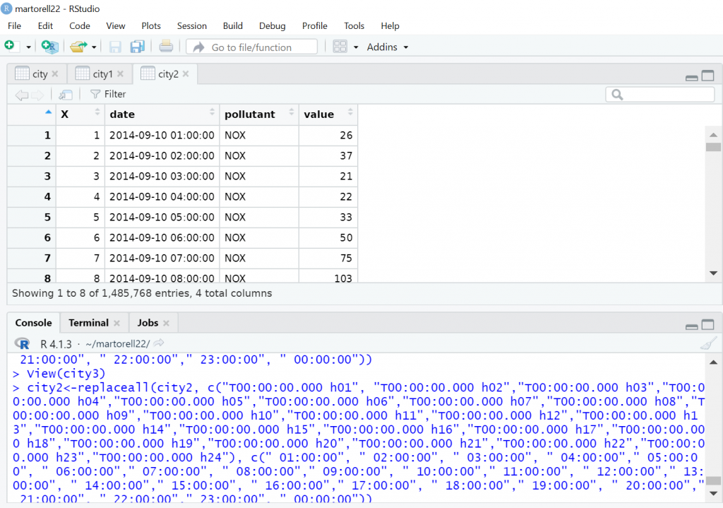
Air pollution data after replaceall instruction in order to obtain data in year-month-day hour: minutes:seconds format in order to apply openair instructions.
CORRELATION IN R
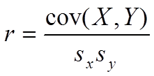
Correlation in graphs
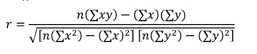
Correlation in formulas
Example: Icecream sales and temperature correlation
Student’s t test (signal/noise ratio) with N-2 degrees of freedom

What is correlation in simple words?
Another example to explain correlation is not causation.


It is very important to draw data in graphs because correlation and other data could be the same (mean, variance, linear relationship), but the data could be very different as in the Anscombe’s quartet.
Linear model
> lm(formula=NO2~NO,data=martorell)
Call:
lm(formula = NO2 ~ NO, data = martorell)
Coefficients:
(Intercept) NO
29.1185 0.3177
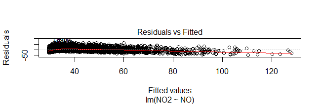
lmfit<-lm(formula=NO2~NO,data=martorell)
> plot(lmfit)Hit <Return> to see next plot:
plot(martorell$NO, martorell$NO2)
> abline(lmfit)
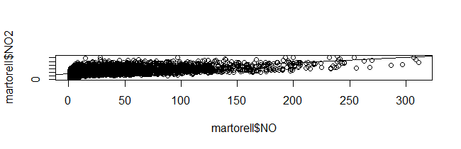
This means that the linear relation is NO2=29.1185+0.3177NO
If you ask for summary(lmfit) you will obtain all this information:
> summary(lmfit)
Call:
lm(formula = NO2 ~ NO, data = martorell)
Residuals:
Min 1Q Median 3Q Max
-49.453 -12.389 -1.978 9.845 84.116
Coefficients:
Estimate Std. Error t value Pr(>|t|)
(Intercept) 29.118529 0.216955 134.21 <2e-16 ***
NO 0.317714 0.004818 65.94 <2e-16 ***
—
Signif. codes: 0 ‘***’ 0.001 ‘**’ 0.01 ‘*’ 0.05 ‘.’ 0.1 ‘ ’ 1
Residual standard error: 16.17 on 8242 degrees of freedom
(540 observations deleted due to missingness)
Multiple R-squared: 0.3454, Adjusted R-squared: 0.3453
F-statistic: 4348 on 1 and 8242 DF, p-value: < 2.2e-16
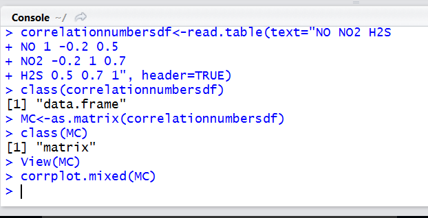
Correlation tests in R
R CODE
> cor.test(martorell$NO,martorell$NO2)
Pearson’s product-moment correlation
data: martorell$NO and martorell$NO2
t = 65.942, df = 8242, p-value < 2.2e-16
alternative hypothesis: true correlation is not equal to 0
95 percent confidence interval:
0.5733714 0.6016387
sample estimates:
cor
0.5876844
This means correlation is 0.59
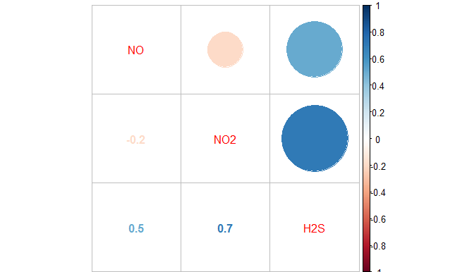
Corrplot R library allows you to graph different correlation coefficients between pollutants
AIR POLLUTION ANALYSIS USING R SOFTWARE
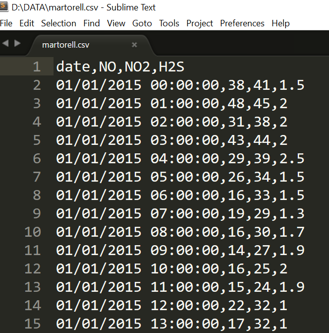
It is very important to use correct comma separated values (csv) files. Remember to save as csv in LibreOffice Calc or Microsoft Office Excel and to replace all commas to points, then all semicolons to commas and finally all Sense dades to NA. After all that you can use your data in R Studio using the instructions found in the table below.
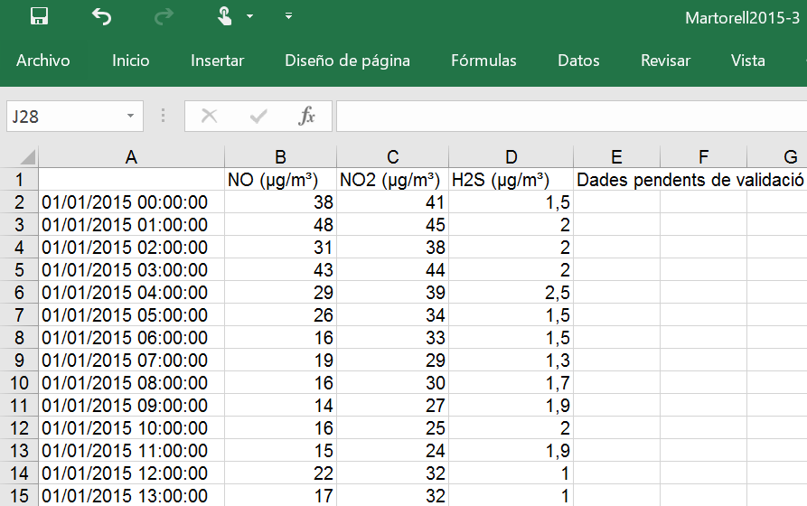
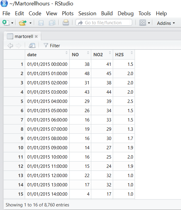
| Read dataframe | martorell<-read.csv(“E://PollutionData/martorell2015.csv”) |
| Calculate quartiles, median, min, max, outliers | summary (martorell) |
| Create boxplot | boxplot(martorell$NO) |
| Create histogram | hist(martorell$NO, breaks=20, xlab=”NO(micrograms/m3)”, main=”Martorell air pollution”, col= “pink”) |
| Install and load normality test | install.packages(” nortest “)
library(nortest)
|
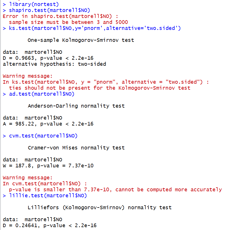
| Shapiro- Wilk normality test
Anderson-Darling normality test Cramer-von-Mises normality test Kolmogorov-Smirnov normality test Pearson normality test Shapiro-Francia normality test |
shapiro.test(martorell$NO)
ad.test(martorell$NO) cvm.test(martorell$NO) lillie.test(martorell$NO) pearson.test(martorell$NO) sf.test(martorell$NO) |
| library (e1071) | skewness(x), kurtosis(x) |
| skewness (negative:left tail, positive: right tail, normal:0) | skewness(martorell$NO) |
| kurtosis (negative : platycurtic, positive : leptocurtic, normal :0) | kurtosis(martorell$NO) |
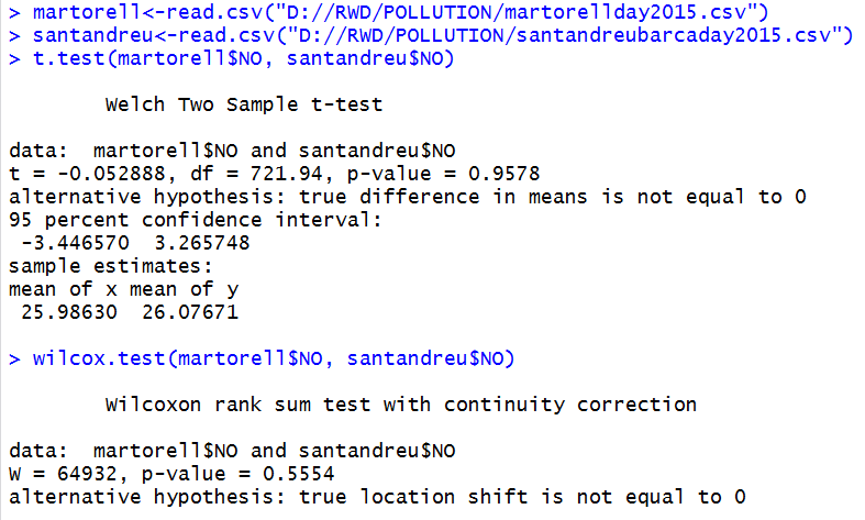
| Student t test (compare 2 normal data) | t.test(martorell$NO, santandreu$NO) |
| U Mann Whitney (compare 2 non normal data) | wilcox.test(martorell$NO, santandreu$NO) |
| Compare > 2 normal groups | ANOVA test |
| Compare > 2 non-normal grous | Kruskal-Wallis test |
| Homocedascity (equal variability) | leveneTest(x) in car library |
| View possible correlation | pairs (martorell) |
| Object type : class (x) | numeric, date, time series, dataframe, etc |
| Convert numeric to date | martorell$date<-as.Date(martorell$date) |
| Create time series | martorellNO.ts <- ts(martorell$NO, start=c(2015, 1, 1), end=c(2015, 12,31), frequency=365) |
| Bind column data | NOcompare<-cbind(martorellNO.ts,santandreuNO.ts) |
| Plotting multiple time series | plot(NOcompare, plot.type=”m”,col=c(“blue”, “red”)) |
| Subset time series | mytssummer2015 <- window(myts, start=c(2015, 6,21), end=c(2015, 9,22)) |
| Correlation plot | library (corrplot)
corrplot.mixed (martorell) |
| Linear model | fit<-lm(martorell$NO~martorell$NO2)
summary(fit) |

Regarding NO2 levels found in previous image:
Is Martorell following the NO2 air pollution standards of the EU?
What is the EU decission 3 about NO2 pollution? In Spanish (authentic and valid)
Analyse all EU air standards and compare to WHO air standards
> plot(martorell$date, martorell$NO, type = "l", xlab = "year 2015",ylab = "Nitric oxide (microg/m3)")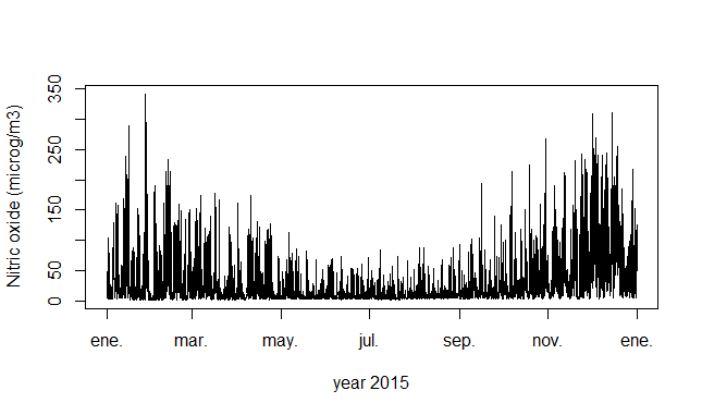
Normality tests
install.packages(“nortest”)
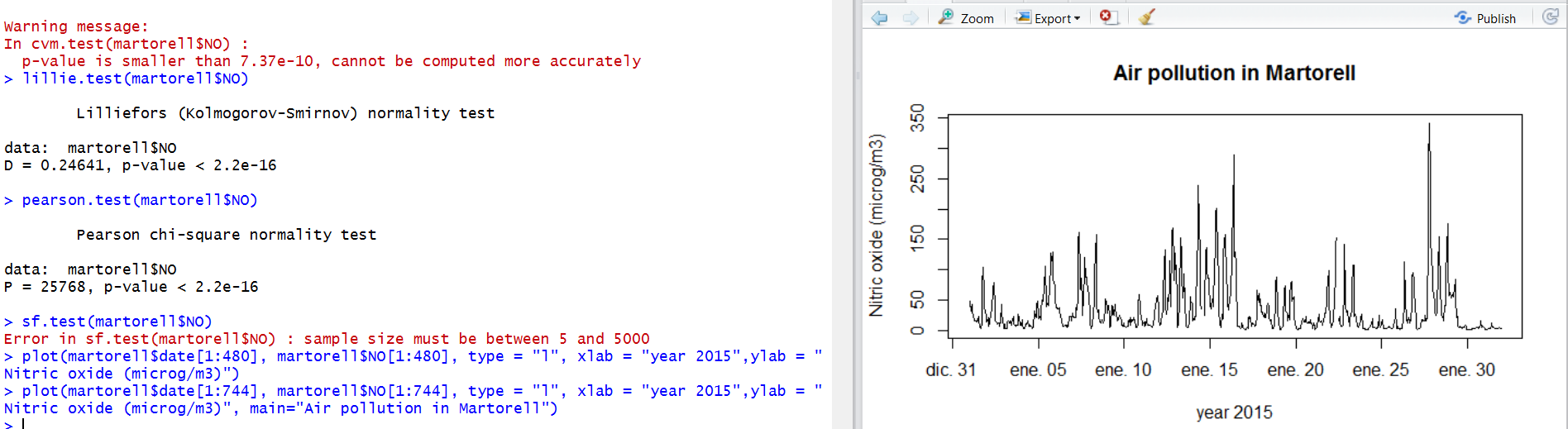
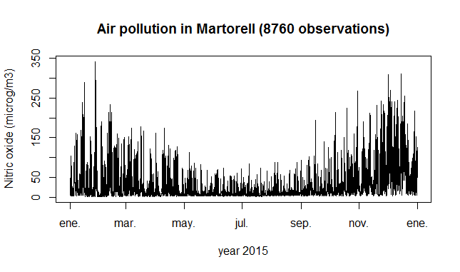
> plot(martorell$date, martorell$NO, type = “l”, xlab = “year 2015”,ylab = “Nitric oxide (microg/m3)”, main=”Air pollution in Martorell (8760 observations)”)
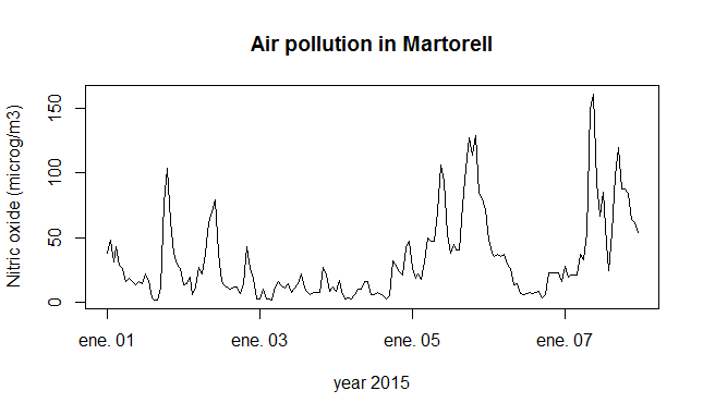
> plot(martorell$date[1:168], martorell$NO[1:168], type = “l”, xlab = “year 2015”,ylab = “Nitric oxide (microg/m3)”, main=”Air pollution in Martorell”)
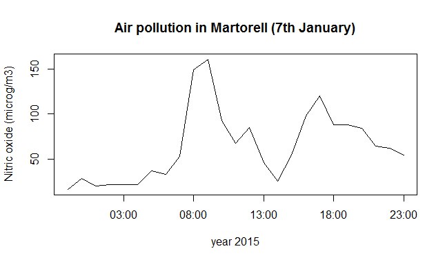
> plot(martorell$date[144:168], martorell$NO[144:168], type = “l”, xlab = “year 2015”,ylab = “Nitric oxide (microg/m3)”, main=”Air pollution in Martorell (7th January)”)
Time series air pollution comparison Martorell vs Sant Andreu de la Barca
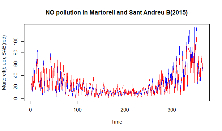
T- test (normal data) or U Mann- Withney (non-normal data)
Air pollutant in Martorell
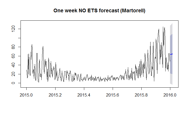
One week forecast of air pollution in Martorell